
This article is transferred from: Reading technology Zouxy finishing
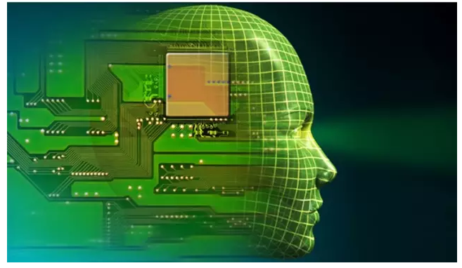
Deep learning , Deep Learning, is a learning algorithm and is also an important branch of artificial intelligence. From rapid development to practical application, deep learning has overturned the algorithm design ideas in many fields such as speech recognition, image classification, and text understanding in just a few years and gradually formed a kind of end-to-end training data. The end-to-end model is then output directly to obtain a new model of the final result. So, how deep is deep learning? Did you learn a bit? This article will take you through the methods and processes behind the deep learning of high-end range.
I. OverviewSecond, background three, human brain vision mechanism four, on the characteristics
4.1. Granularity of Feature Representation 4.2. Primary (Shallow) Feature Representation 4.3. Structural Feature Representation 4.4. How Many Characteristics Do We Need? V. The basic ideas of Deep Learning VI. Shallow Learning and Deep Learning 7. Deep Learning and Neural Network 8. Deep Learning Training Process 8.1. Traditional Neural Network Training Methods 8.2. Deep Learning Training Process Nine, commonly used models or methods of Deep Learning 9.1, AutoEncoder automatic encoder 9.2, Sparse Coding sparse coding 9.3, Restricted Boltzmann Machine (RBM) restrictions Boltzmann machine 9.4, Deep BeliefNetworks deep belief network 9.5, Convolutional Neural Networks convolutional nerve Network Ten, Summary and Outlook
| I. Overview
Artificial Intelligence, also known as human intelligence, is one of humankind's best dreams, just like immortality and interplanetary roaming. Although computer technology has made great progress, so far, there is not a computer that can generate "self" consciousness. Yes, with the help of humans and a large amount of ready-made data, the computer can perform very powerfully, but leaving the two, it can't even tell a comet and a Wangxing.
Turing (Turing, we all know it. The originators of computers and artificial intelligence, corresponding to their famous Turing machines and Turing tests, respectively) proposed in the 1950 paper that the Turing experiment envisaged Dialogue with the wall, you will not know whether to talk to you, people or computers. This undoubtedly gives computers, especially artificial intelligence, a preset high expectation. But half a century has passed and the progress of artificial intelligence is far from reaching the Turing test standard. This is not only disappointing people who have been waiting for years, but also believes that artificial intelligence is a flicker and related fields are "pseudoscience."
However, since 2006, the field of machine learning has made breakthrough progress. The Turing experiment was at least not as far-reaching as possible. As for technical means, not only rely on the ability of cloud computing for parallel processing of big data, but also rely on algorithms. The algorithm is, Deep Learning. With the help of the Deep Learning algorithm, humans finally found a way to deal with the ancient concept of "abstract concept."
In June 2012, the "New York Times" disclosed the Google Brain project and attracted wide public attention. The project was led by Andrew Ng, a renowned Stanford University professor of machine learning, and Jeff Dean, a world-leading expert in large-scale computer systems. He trained a so-called "deep neural network" (DNN) using a parallel computing platform of 16,000 CPU Cores. , Deep Neural Networks' machine learning model (having a total of 1 billion nodes internally. This network naturally cannot be compared with human neural networks. It should be noted that there are more than 15 billion neurons in the human brain, interconnected nodes That is, the number of synapses is more like the number of galactic sands. It has been estimated that if the axons and dendrites of all nerve cells in a person’s brain are connected in sequence and pulled into a straight line, they can be connected from the earth to the moon. Returning to Earth from the Moon, it achieved great success in the fields of speech recognition and image recognition.
Andrew, one of the project leaders, said: "We didn't frame our boundaries like we usually do, but we put a lot of data directly into the algorithm, let the data speak for itself, and the system automatically learns from the data." Another person in charge Jeff said: "We never told the machine when we were training that: 'This is a cat.' The system actually invented or understood the concept of 'cat'."

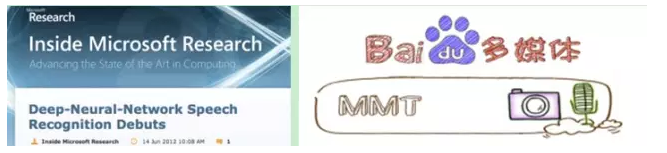
In November 2012, Microsoft publicly demonstrated a fully automated simultaneous interpretation system at an event in Tianjin, China. The lecturer gave a speech in English. The computer in the background automatically completed speech recognition, English-Chinese machine translation, and Chinese speech synthesis. Very smooth. According to reports, the key technology behind the support is also DNN, or Deep Learning (DL, DeepLearning).
In January 2013, at Baidu's annual meeting, founder and CEO Robin Li announced a high-profile announcement of the establishment of Baidu Research Institute, the first of which was the Institute of Deep Learning (IDL).
Why do Internet companies with big data rush to invest heavily in research and development of deep learning technologies. It sounds like deeplearning like cows. What is deep learning? Why deep learning? How did it come from? What can you do? What are the current difficulties? The brief answers to these questions need to be taken slowly. Let's first understand the background of machine learning (the core of artificial intelligence).
| Second, background
Machine Learning is a discipline that specializes in how computers simulate or realize human learning behavior to acquire new knowledge or skills and reorganize existing knowledge structures to continuously improve their performance. Can machines be as capable as humans? In 1959, Samuel of the United States designed a chess program. This program has the ability to learn. It can improve his chess skills in continuous chess. Four years later, this program defeated the designer himself. After another three years, this procedure defeated the United States, an undefeated champion who has maintained an eight-year history. This program shows people the ability of machine learning, and put forward many thought-provoking social issues and philosophical issues. (Oh, the normal track of artificial intelligence has not been greatly developed. What these philosophical ethics have developed very quickly. What is the future? Machines are more and more like people, people are more and more like machines. What machines are anti-human, ATM is the first shot, etc. The human mind is endless.)
Although machine learning has developed for decades, there are still many problems that are not well solved:
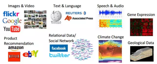
For example, image recognition, speech recognition, natural language understanding, weather prediction, gene expression, content recommendation, and the like. At the moment, we are thinking of solving these problems through machine learning (visual perception as an example):
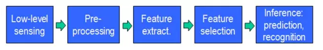
Data is obtained from the beginning through a sensor (for example, CMOS). Then after preprocessing, feature extraction, feature selection, and then to reasoning, prediction or identification. The last part, that is, the part of machine learning, the vast majority of the work is done in this area, there are a lot of paper and research.
The middle three parts are summarized as feature expressions. The good feature expression plays a very key role in the accuracy of the final algorithm, and the system's main calculation and testing work consumes most of this. However, this practice is generally done manually. Rely on artificial extraction features.
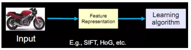
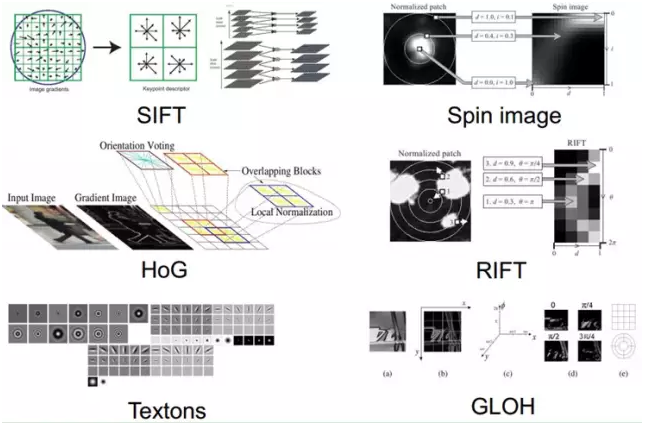
As of now, there have been many characteristics of NB (good features should have invariance (size, scale, rotation, etc.) and distinguishability): For example, the emergence of Sift is a landmark in the field of local image feature descriptor research. work. Because SIFT is invariant to image changes such as scale, rotation and certain angles of view and illumination changes, and SIFT is very distinguishable, it does make it possible to solve many problems. But it is not everything.
However, the manual selection of features is a very laborious and heuristic (requiring professional knowledge) approach. Whether or not it can be selected depends largely on experience and luck, and its adjustment requires a lot of time. Since manual selection of features is not so good, can we learn some features automatically? The answer is yes! Deep Learning is used to do this. Look at it as an alias UnsupervisedFeature Learning, you can justify the name, Unsupervised means that people do not participate in the selection process.
How did it learn? How do you know which features are better or not? We say that machine learning is a discipline that specializes in how computers simulate or realize human learning behavior. Well, how does our human visual system work? Why can we find another one in the vast sea, the mortal beings, the red dust (because you exist in my deep mind, my dreams my heart my song ...). The human brain then NB, can we refer to the human brain and simulate the human brain? (It seems to be related to the characteristics of the human brain, ah, the algorithm is good, but I do not know whether it is artificially imposed, in order to make his work sacred and elegant.) In recent decades, cognitive neuroscience The development of disciplines such as biology and biology has made us no longer unfamiliar with our mysterious and magical brain. It also contributed to the development of artificial intelligence.
| Third, the human brain vision mechanism
The 1981 Nobel Prize in Medicine was awarded to David Hubel (American neurobiologist born in Canada) and Torsten Wiesel, and Roger Sperry. The main contributions of the first two are "discovery of information processing in the visual system": The visual cortex is graded:
Let's see what they have done. In 1958, David Hubel and Torsten Wiesel at John Hopkins University studied the correspondence between the pupil area and the cerebral cortical neurons. They opened a 3mm hole in the cat's hindbrain skull and inserted electrodes into the hole to measure the activity of the neurons.
Then, in front of the cat's eyes, they showed various shapes and various brightness objects. And, when presenting each object, it also changes the position and angle at which the object is placed. They hope that through this approach, the kitten's pupils will experience different types of different strengths and irritations.
The reason for doing this experiment is to prove a guess. There is a corresponding relationship between different visual neurons located in the posterior cortex and the stimulation of the pupil. Once the pupil is stimulated, a certain part of the neurons in the posterior cortex will become active. After many days of tedious experiments and sacrifices of poor kittens, David Hubel and Torsten Wiesel discovered a type of neuron called the Orientation Selective Cell. When the pupil finds the edge of the object in front of the eye and the edge points in a certain direction, the neuron cell becomes active.
This discovery inspired people to think further about the nervous system. The working process of the nerve-center-brain may be an iterative, continuous abstraction process. There are two keywords here, one is abstraction and the other is iteration. From the original signal, do low-level abstractions and gradually iterate to high-level abstractions. Human logical thinking often uses highly abstract concepts.
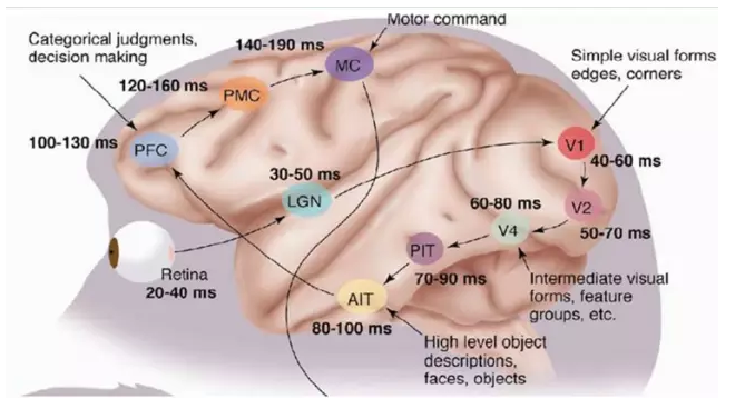
For example, starting from the original signal intake (pupil uptake pixel Pixels), then doing preliminary processing (cerebral cortex some cells find the edge and direction), then abstract (the brain determines that the shape of the object in front of the eyes, is round) Then further abstraction (the brain further determines that the object is a balloon).
The discovery of this physiology contributed to the breakthrough of computer artificial intelligence in 40 years.
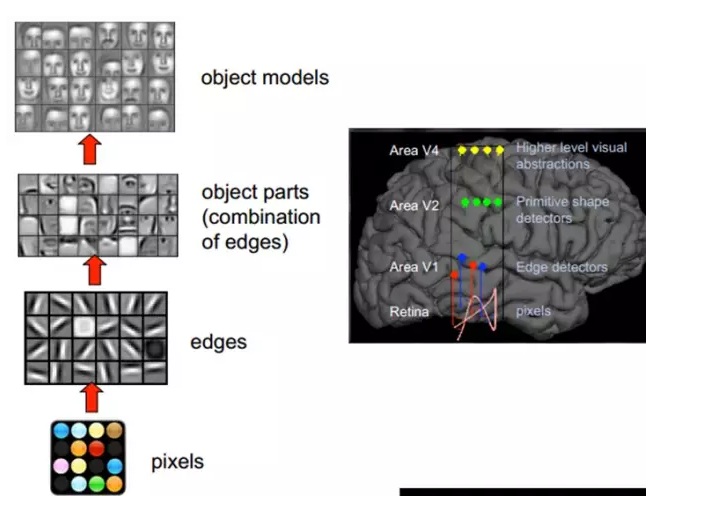
In general, the information processing of the human visual system is hierarchical. From the low-level V1 area to extract edge features, to the shape of the V2 area or part of the target, etc., to the higher level, the entire target, the behavior of the target. In other words, the high-level features are the combination of low-level features. From the low-level to the high-level, feature representations become more and more abstract, and they can express semantics or intentions more and more. The higher the level of abstraction, the fewer possible guesses there are and the better it is for classification. For example, the correspondence between word sets and sentences is many-to-one, and the correspondence between sentences and semantics is many-to-one, and the correspondence between semantics and intentions is many-to-one. This is a hierarchical system.
Sensitive people notice the key word: stratification. Is Deep learning deep enough to indicate how many layers I have, and how deep is it? That's right. How does Deep learning learn from this process? After all, it is due to the computer to deal with. The problem is how to model this process?
Because we want to learn the expression of characteristics, then we need to understand more about the characteristics, or about the characteristics of the hierarchy. So before we say Deep Learning, it is necessary for us to write down the features. (Oh, actually seeing such a good explanation of the features is not a pity here, so we plug it here).
| IV. About Features
The feature is the raw material of the machine learning system, and the impact on the final model is beyond doubt. If the data is well expressed as a feature, the linear model can usually achieve satisfactory accuracy. What do we need to consider for features?
4.1, the granularity of the feature representation
What is the granularity of the learning algorithm's characteristics that can play a role? In terms of a picture, pixel-level features have no value at all. For example, the motorcycle below does not receive any information at all from the pixel level, and it cannot distinguish between motorcycles and non-motorcycles. If the feature is a structural (or meaningful) time, such as whether it has a handlebar and whether it has a wheel, it is easy to distinguish the motorcycle from the non-motorcycle, and the learning algorithm can work. .

4.2 Primary (Shallow) Feature Representation
Since pixel-level feature representation does not work, what kind of representation is useful?
Around 1995, two scholars, Bruno Olshausen and David Field, worked at Cornell University. They tried to use physiology and computers to study visual problems in a two-pronged approach. They collected a lot of black and white landscape photos. From these photos, 400 small pieces were extracted. The size of each photo was 16x16 pixels. Mark the 400 pieces as S[i], i = 0, .. 399. Next, from the black and white landscape photos, another fragment is randomly extracted, and the size is also 16x16 pixels. You may wish to mark this fragment as T.
The question they asked was how to select a set of fragments from the 400 fragments, S[k], and synthesize a new fragment by stacking. This new fragment should be randomly selected with the target fragment T , as similar as possible, while the number of S[k] is as small as possible. Described in the language of mathematics, is:
Sum_k (a[k]S[k]) --> T, where a[k] is the weight coefficient when the fragment S[k] is superimposed.
To solve this problem, Bruno Olshausen and David Field invented an algorithm, sparse coding (Sparse Coding).
Sparse coding is a repeated iterative process with two steps per iteration:
1) Select a set of S[k] and adjust a[k] so that Sum_k(a[k]S[k]) is closest to T.
2) Fix a[k]. Among the 400 fragments, select other more suitable fragments S'[k], replacing the original S[k], making Sum_k (a[k]S'[k]) the closest T.
After several iterations, the best S[k] combination was selected. Surprisingly, the selected S[k] is basically the edge line of the different objects on the photo. These line segments are similar in shape and differ in direction.
The algorithmic results of Bruno Olshausen and David Field coincide with the physiological findings of David Hubel and Torsten Wiesel!
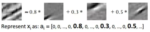
In other words, complex graphics often consist of some basic structure. For example, the following figure shows a graph that can be represented linearly by using 64 orthogonal edges, which can be understood as orthogonal basic structures. For example, the sample x can be reconstructed by using the weights of 0.8, 0.3, and 0.5 from three out of 1-64 edges. The other basic edges do not contribute and are therefore 0.
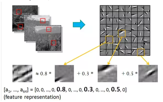
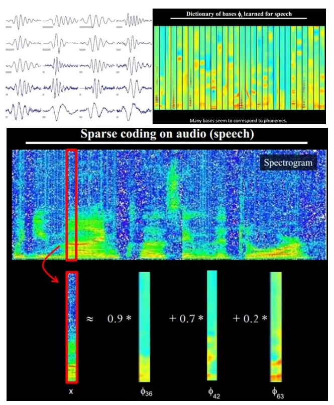
In addition, the big cows also found that not only the law exists in the images, but also sounds exist. They have discovered 20 basic sound structures from unmarked sounds, and the rest of the sounds can be synthesized from these 20 basic structures.
4.3. Representation of structural features
Small pieces of graphics can be made up of basic edges, more structured, more complex, and how do the conceptual graphics be represented? This requires a higher level of feature representation, such as V2, V4. Therefore, V1 looks at the pixel level as a pixel level. V2 sees V1 as a pixel level. This is a hierarchical progression. High-level expressions are formed by a combination of underlying expressions. Professionalism is the basic basis. V1 assumes that the base is the edge, and then the V2 layer is the combination of these bases of the V1 layer. At this time, the V2 area obtains a higher level of base. That is, the result of the combination of the upper layers is the combination of the upper layer and the upper layer... (Therefore, Da Ng said that Deep Learning is the "base", because it is ugly, so its name is Deep Learning or Unsupervised Feature Learning. )

Intuitively speaking, it is to find the small patch of make sense and then combine it to get the upper layer of features, recursively upward learning feature.
When doing training on different objects, the resulting edgebasis is very similar, but the object parts and models will be completely different (that's how easy it is to distinguish car or face):

From the text, what does a doc mean? We describe one thing. What does it mean to be more appropriate? With a word, I don't see it. The word is pixel level. At least it should be a term. In other words, each doc is made up of a term, but the ability to express the concept is enough, and it may not be enough. One step, reaching the topic level, with the topic, and then to the doc is reasonable. However, there is a large gap between the levels of each level, such as the concept of doc -> topic (thousands of thousands - million) -> term (10 million) -> word (million level).
When a person is looking at a doc, what his eyes see is word. Words are automatically word-formed in the brain to form term. In the way of concept organization, prior learning, topic, and then high-level learning .
4.4 How many features do I need?
We know that there needs to be a hierarchy of feature construction, from shallow to deep, but how many features should there be in each layer?
The more features, the more reference information given and the accuracy will be improved. However, multiple features means that the calculation is complex and the exploration space is large. The data that can be used for training will be sparse in each feature and will bring about various problems. The more features, the better.
Well, at this point, we can finally talk about Deep learning. Above we talked about why there is Deep learning (which allows the machine to automatically learn good features, and eliminate the manual selection process and the reference layered visual processing system). We have come to the conclusion that Deep learning requires multiple layers to obtain more Abstract feature expression. How many layers are appropriate? What architecture is used to model it? How to conduct non-supervisory training?
| V. The basic idea of ​​Deep Learning
Suppose we have a system S, which has n layers (S1,...Sn), whose input is I and whose output is O, which is visually represented as: I => S1 => S2 =>..... => Sn => O, if the output O is equal to the input I, that is, after the input I has undergone this system change, there is no information loss (Oh, Da Niu said, this is not possible. Information theory has a saying that "information is lost layer by layer" (information processing Inequality), suppose that processing a information to obtain b, and then b processing to obtain c, then we can prove: a and c mutual information will not exceed the mutual information of a and b. This shows that information processing will not increase information, most of the processing will Loss of information. Of course, if it is worthless to lose information that is useless, and it stays the same, this means that input I goes through every layer of Si without any loss of information, ie, at any level of Si, it It is another representation of the original information (ie input I). Now back to our theme Deep Learning, we need to learn features automatically. Suppose we have a bunch of input I (like a bunch of images or text). Suppose we have designed a system S (with n layers). We adjust the parameters in the system. So that its output is still input I, then we can automatically get a series of hierarchical features of the input I, namely S1, ..., Sn.
For deep learning, the idea is to stack multiple layers, that is, the output of this layer as the input to the next layer. In this way, it is possible to hierarchically express the input information.
In addition, the front is assuming that the output is strictly equal to the input. This limit is too strict. We can slightly relax this limit. For example, we only need to make the difference between input and output as small as possible. This relaxation will lead to another type of different Deep. Learning method. The above is the basic idea of ​​Deep Learning.
| 6. Shallow Learning and Deep Learning
Shallow learning is the first wave of machine learning.
In the late 1980s, the invention of the back-propagation algorithm (also called Back Propagation algorithm or BP algorithm) for artificial neural networks brought hope to machine learning and set off an upsurge of machine learning based on statistical models. This boom continued until today. It has been found that using the BP algorithm allows an artificial neural network model to learn statistical rules from a large number of training samples and thus predict unknown events. This kind of statistics-based machine learning method has superiority in many aspects compared with the past based on artificial rules. Artificial neural network at this time, although also known as Multi-layer Perceptron, is actually a shallow model containing only one hidden layer node.
In the 1990s, a variety of shallow machine learning models were successively proposed, such as Support Vector Machines (SVM), Boosting, and Maximum Entropy methods (such as LR, Logistic Regression). The structure of these models can basically be seen as a hidden layer node (such as SVM, Boosting), or no hidden layer nodes (such as LR). These models have achieved great success both in theoretical analysis and in their application. In contrast, due to the difficulty of theoretical analysis, training methods also require a lot of experience and skills. During this period, shallow artificial neural networks are relatively quiet.
Deep learning is the second wave of machine learning.
In 2006, Professor Geoffrey Hinton and his student Ruslan Salakhutdinov of the University of Toronto, Canada, and his student Ruslan Salakhutdinov published an article in Science that opened the wave of deep learning in academia and industry. This article has two main viewpoints: 1) The multi-hidden layer artificial neural network has excellent feature learning capabilities, and the learned features have a more characterization of the data, which is conducive to visualization or classification; 2) deep neural networks Difficulties in training can be effectively overcome by layer-wise pre-training. In this article, layer-by-layer initialization is achieved through unsupervised learning.
Currently, most of the learning methods such as classification and regression are shallow structure algorithms. The limitation is that the ability to represent complex functions is limited in the case of finite samples and computational units, and the generalization ability of complex classification problems is restricted. Deep learning can learn a deep nonlinear network structure, realize the approximation of complex functions, represent the distributed representation of input data, and demonstrate a strong ability to learn the essential characteristics of data sets from a few sample sets. (The advantage of multi-layer is that you can express complex functions with fewer parameters.)

The essence of deep learning is to learn more useful features by constructing a machine learning model with a lot of hidden layers and massive training data, so as to ultimately improve the accuracy of classification or prediction. Therefore, "deep model" is the means, and "characteristic learning" is the purpose. Different from traditional shallow learning, the difference in deep learning is that: 1) The depth of the model structure is emphasized, usually 5, 6 or even 10 layers of hidden layer nodes; 2) The importance of feature learning is clearly highlighted That is to say, through layer-by-layer feature transformation, the feature representation of the sample in the original space is transformed into a new feature space, thereby making classification or prediction easier. Compared with the method of constructing features by artificial rules, using big data to learn features makes it possible to describe the rich internal information of data.
| VII, Deep learning and Neural Network
Deep learning is a new field in machine learning research. Its motivation lies in building and simulating the neural network of the human brain for analytical learning. It imitates the mechanism of the human brain to interpret data such as images, sounds, and texts. Deep learning is a kind of unsupervised learning.
The concept of deep learning stems from the study of artificial neural networks. A multilayer sensor with multiple hidden layers is a deep learning structure. Deep learning creates more abstract high-level representation attribute categories or features by combining low-level features to discover distributed representations of data.
Deep learning itself is a branch of machine learning. Simple can be understood as the development of neural networks. About two or three decades ago, neural network was once a particularly hot direction in the ML field, but it has since slowly faded out. The reasons include the following aspects:
1) It is easier to overfit, the parameters are more difficult to tune, and many tricks are needed;
2) The training speed is slow, and the effect is not better than other methods when the level is relatively small (less than or equal to 3);
So for about 20 years in the middle, the neural network was little noticed. This time is basically the world of SVM and boosting algorithms. However, an infatuated old Mr. Hinton, he persisted, and finally (and others Bengio, Yann.lecun, etc.) into a practical deep learning framework.
There are many differences between Deep learning and traditional neural networks.
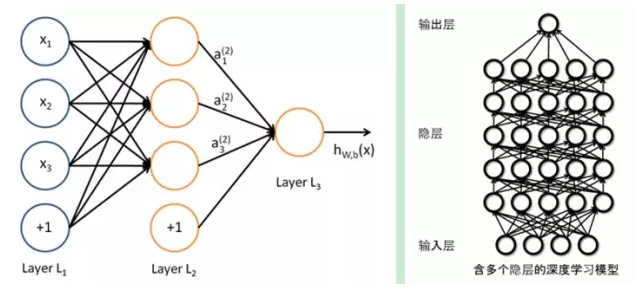
The difference between the two is that deep learning adopts a similar hierarchical structure of neural networks. The system consists of a multi-layer network consisting of input layer, hidden layer (multi-layer), and output layer. Only the adjacent layer nodes have connections, the same layer. And cross-layer nodes are not connected to each other, each layer can be seen as a logistic regression model; this hierarchical structure is closer to the structure of the human brain.
In order to overcome the problems in neural network training, DL adopts a very different training mechanism from neural networks. In the traditional neural network, the method of back propagation is adopted. In simple terms, an iterative algorithm is used to train the entire network, the initial value is set at random, the output of the current network is calculated, and then the difference between the current output and the label is used. Change the parameters of the previous layers until convergence (the whole is a gradient descent method). Deep learning as a whole is a layer-wise training mechanism. The reason for this is because, if the back propagation mechanism is used, for a deep network (more than 7 layers), the residual spread to the frontmost layer has become too small, with the so-called gradient diffusion. We will discuss this issue next.
| Eight, deep learning training process
8.1. Why can't traditional neural network training methods be used in deep neural networks?
BP algorithm is a typical algorithm for traditional training multi-layer networks. In fact, it only contains several layers of networks. This training method is already very unsatisfactory. The ubiquitous local minimum in the non-convex target cost function of the deep structure (involving multiple nonlinear processing unit layers) is the main source of training difficulties.
Problems with the BP algorithm:
(1) Gradient is becoming sparse: the error correction signal is getting smaller and smaller from the top down;
(2) Convergence to local minimums: especially when starting from far away from the optimal region (initialization of random values ​​will cause this to happen);
(3) In general, we can only train with tagged data: but most of the data is unlabeled, and the brain can learn from untagged data;
8.2, deep learning training process
If you train all layers at the same time, the time complexity will be too high; if you train one layer at a time, the deviation will be passed layer by layer. This will face the opposite problem of supervised learning above, and it will seriously under-fit (because the depth of the network has too many neurons and parameters).
In 2006, Hinton proposed an effective method for building multi-layer neural networks on unsupervised data. In simple terms, there are two steps. One is to train one network at a time, and the other is to tune the original representation x upwards. The high-level representation r and the high-level representation r are as consistent as possible. the way is:
1) First build a single layer of neurons layer by layer, so that each time you train a single-layer network.
2) After all layers have been trained, Hinton uses the wake-sleep algorithm for tuning.
Turn the weights of the layers except the topmost layer into bidirectional, so that the top layer is still a single-layer neural network, and other layers become the graph model. The upward weight is used for "cognitive" and the downward weight is used for "generating." Then use the Wake-Sleep algorithm to adjust all the weights. The consensus between cognition and generation is to ensure that the generated top-level representation can restore the underlying nodes as correctly as possible. For example, if a node at the top level represents the face, then the image of all faces should activate the node, and the resulting downward-looking image should be able to appear as a general face image. Wake-Sleep algorithm is divided into wake and sleep.
1) Wake phase: The cognitive process generates an abstract representation of each layer (node ​​state) through external features and upward weights (cognitive weights), and uses gradient descent to modify the downlink weight between layers (generate weights). That is, "If the reality is different from what I have imagined, changing my weight makes my imagination something like this."
2) sleep stage: the generation process, through the top-level representation (concept learned when awake) and down the weight, to generate the underlying state, while modifying the upward weight between layers. That is, "if the dream scene is not a corresponding concept in my mind, changing my cognitive weight makes this scene seem to me the concept."
The deep learning training process is as follows:
1) Use non-supervised learning from the bottom up (that is, start from the ground up, layer by layer to top level training):
Using non-calibrated data (with calibration data also available) to stratify parameters at each level, this step can be seen as an unsupervised training process, which is the most distinct part from the traditional neural network (this process can be seen as a feature learning process)
Specifically, the first layer is first trained with no calibration data, and the parameters of the first layer are learned first (this layer can be seen as a hidden layer of a three-layer neural network that minimizes the difference between output and input). The limitation of capacity and the sparsity constraint make the obtained model able to learn the structure of the data itself, so as to obtain features that are more capable of expressing than the input; after learning to obtain the n-1th layer, the output of the n-1 layer is taken as the first The n-layer input trains the n-th layer, from which each layer's parameters are obtained;
2) Top-down supervised learning (that is, training with tagged data, error propagation from the top, fine-tuning the network):
Based on the parameters obtained in the first step to further fine-tune the parameters of the entire multi-layer model, this step is a supervised training process; the first step is similar to the neural network's random initialization initial value process, since the first step of DL is not random Initialization, but obtained by learning the structure of the input data, so that the initial value is closer to the global optimum, so that better results can be achieved; so the deep learning effect is largely due to the first step of the feature learning process.
| Nine, Deep Learning common model or method
9.1, AutoEncoder Automatic Encoder
One of the simplest methods of Deep Learning is to use the characteristics of artificial neural networks. An artificial neural network (ANN) is itself a system with a hierarchical structure. If a neural network is given, we assume that its output and input are the same, and then training adjustments. Its parameters get the weight in each layer. Naturally, we get several different representations of input I (each layer represents a representation), and these representations are features. An automatic encoder is a neural network that reproduces the input signal as much as possible. In order to achieve this kind of reproduction, the automatic encoder must capture the most important factor that can represent the input data, just like the PCA, find the main component that can represent the original information.
The specific process is briefly described as follows:
1) Given unlabeled data, learn features using unsupervised learning:

In our previous neural network, as in the first diagram, the input sample is labeled, ie, (input, target), so that we change the previous layers according to the difference between the current output and the target(label). Parameters until convergence. But now we only have unlabeled data, which is the figure on the right. How can this error be obtained?
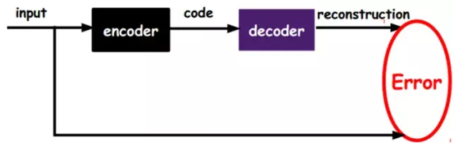
As shown above, we will input an input encoder encoder, you will get a code, this code is a representation of the input, then how do we know this code is input it? We add a decoder decoder. At this time, the decoder will output a message. If the output information is similar to the input signal input (ideally, it is the same), it is obvious that we have a reason. I believe this code is reliable.所以,我们就通过调整encoderå’Œdecoderçš„å‚数,使得é‡æž„误差最å°ï¼Œè¿™æ—¶å€™æˆ‘们就得到了输入inputä¿¡å·çš„第一个表示了,也就是编ç codeäº†ã€‚å› ä¸ºæ˜¯æ— æ ‡ç¾æ•°æ®ï¼Œæ‰€ä»¥è¯¯å·®çš„æ¥æºå°±æ˜¯ç›´æŽ¥é‡æž„åŽä¸ŽåŽŸè¾“入相比得到。

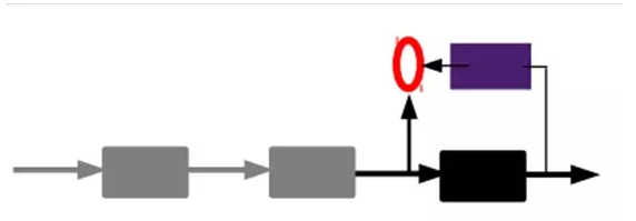
2)通过编ç 器产生特å¾ï¼Œç„¶åŽè®ç»ƒä¸‹ä¸€å±‚ã€‚è¿™æ ·é€å±‚è®ç»ƒï¼š
那上é¢æˆ‘们就得到第一层的code,我们的é‡æž„误差最å°è®©æˆ‘们相信这个code就是原输入信å·çš„良好表达了,或者牵强点说,它和原信å·æ˜¯ä¸€æ¨¡ä¸€æ ·çš„(表达ä¸ä¸€æ ·ï¼Œåæ˜ çš„æ˜¯ä¸€ä¸ªä¸œè¥¿ï¼‰ã€‚é‚£ç¬¬äºŒå±‚å’Œç¬¬ä¸€å±‚çš„è®ç»ƒæ–¹å¼å°±æ²¡æœ‰å·®åˆ«äº†ï¼Œæˆ‘们将第一层输出的code当æˆç¬¬äºŒå±‚的输入信å·ï¼ŒåŒæ ·æœ€å°åŒ–é‡æž„误差,就会得到第二层的å‚数,并且得到第二层输入的code,也就是原输入信æ¯çš„第二个表达了。其他层就åŒæ ·çš„方法炮制就行了(è®ç»ƒè¿™ä¸€å±‚,å‰é¢å±‚çš„å‚数都是固定的,并且他们的decoderå·²ç»æ²¡ç”¨äº†ï¼Œéƒ½ä¸éœ€è¦äº†ï¼‰ã€‚
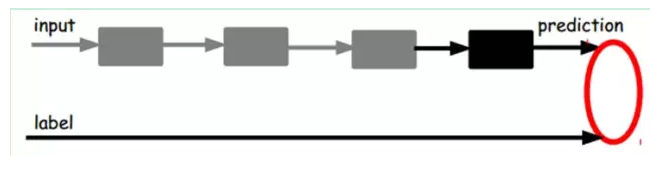
3)有监ç£å¾®è°ƒï¼š
ç»è¿‡ä¸Šé¢çš„方法,我们就å¯ä»¥å¾—到很多层了。至于需è¦å¤šå°‘层(或者深度需è¦å¤šå°‘,这个目å‰æœ¬èº«å°±æ²¡æœ‰ä¸€ä¸ªç§‘å¦çš„评价方法)需è¦è‡ªå·±è¯•éªŒè°ƒäº†ã€‚æ¯ä¸€å±‚都会得到原始输入的ä¸åŒçš„表达。当然了,我们觉得它是越抽象越好了,就åƒäººçš„è§†è§‰ç³»ç»Ÿä¸€æ ·ã€‚
到这里,这个AutoEncoder还ä¸èƒ½ç”¨æ¥åˆ†ç±»æ•°æ®ï¼Œå› 为它还没有å¦ä¹ 如何去连结一个输入和一个类。它åªæ˜¯å¦ä¼šäº†å¦‚何去é‡æž„或者å¤çŽ°å®ƒçš„输入而已。或者说,它åªæ˜¯å¦ä¹ 获得了一个å¯ä»¥è‰¯å¥½ä»£è¡¨è¾“入的特å¾ï¼Œè¿™ä¸ªç‰¹å¾å¯ä»¥æœ€å¤§ç¨‹åº¦ä¸Šä»£è¡¨åŽŸè¾“入信å·ã€‚那么,为了实现分类,我们就å¯ä»¥åœ¨AutoEncoder的最顶的编ç å±‚æ·»åŠ ä¸€ä¸ªåˆ†ç±»å™¨ï¼ˆä¾‹å¦‚ç½—æ°æ–¯ç‰¹å›žå½’ã€SVMç‰ï¼‰ï¼Œç„¶åŽé€šè¿‡æ ‡å‡†çš„多层神ç»ç½‘络的监ç£è®ç»ƒæ–¹æ³•ï¼ˆæ¢¯åº¦ä¸‹é™æ³•ï¼‰åŽ»è®ç»ƒã€‚
也就是说,这时候,我们需è¦å°†æœ€åŽå±‚的特å¾code输入到最åŽçš„åˆ†ç±»å™¨ï¼Œé€šè¿‡æœ‰æ ‡ç¾æ ·æœ¬ï¼Œé€šè¿‡ç›‘ç£å¦ä¹ 进行微调,这也分两ç§ï¼Œä¸€ä¸ªæ˜¯åªè°ƒæ•´åˆ†ç±»å™¨ï¼ˆé»‘色部分):
å¦ä¸€ç§ï¼šé€šè¿‡æœ‰æ ‡ç¾æ ·æœ¬ï¼Œå¾®è°ƒæ•´ä¸ªç³»ç»Ÿï¼šï¼ˆå¦‚果有足够多的数æ®ï¼Œè¿™ä¸ªæ˜¯æœ€å¥½çš„。end-to-end learning端对端å¦ä¹ )
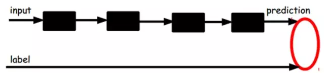
一旦监ç£è®ç»ƒå®Œæˆï¼Œè¿™ä¸ªç½‘络就å¯ä»¥ç”¨æ¥åˆ†ç±»äº†ã€‚神ç»ç½‘络的最顶层å¯ä»¥ä½œä¸ºä¸€ä¸ªçº¿æ€§åˆ†ç±»å™¨ï¼Œç„¶åŽæˆ‘们å¯ä»¥ç”¨ä¸€ä¸ªæ›´å¥½æ€§èƒ½çš„分类器去å–ä»£å®ƒã€‚åœ¨ç ”ç©¶ä¸å¯ä»¥å‘现,如果在原有的特å¾ä¸åŠ 入这些自动å¦ä¹ 得到的特å¾å¯ä»¥å¤§å¤§æ高精确度,甚至在分类问题ä¸æ¯”ç›®å‰æœ€å¥½çš„分类算法效果还è¦å¥½ï¼
AutoEncoderå˜åœ¨ä¸€äº›å˜ä½“,这里简è¦ä»‹ç»ä¸‹ä¸¤ä¸ªï¼š
Sparse AutoEncoder稀ç–自动编ç 器:
当然,我们还å¯ä»¥ç»§ç»åŠ 上一些约æŸæ¡ä»¶å¾—到新的Deep Learning方法,如:如果在AutoEncoderçš„åŸºç¡€ä¸ŠåŠ ä¸ŠL1çš„Regularityé™åˆ¶ï¼ˆL1主è¦æ˜¯çº¦æŸæ¯ä¸€å±‚ä¸çš„节点ä¸å¤§éƒ¨åˆ†éƒ½è¦ä¸º0,åªæœ‰å°‘æ•°ä¸ä¸º0,这就是Sparseåå—çš„æ¥æºï¼‰ï¼Œæˆ‘们就å¯ä»¥å¾—到Sparse AutoEncoder法。
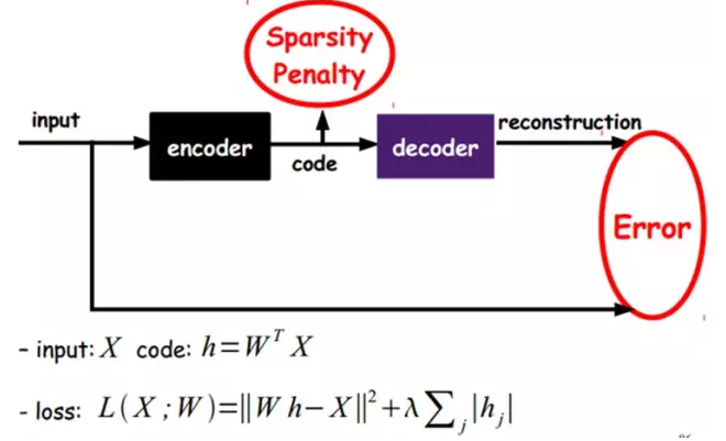
如上图,其实就是é™åˆ¶æ¯æ¬¡å¾—到的表达codeå°½é‡ç¨€ç–ã€‚å› ä¸ºç¨€ç–的表达往往比其他的表达è¦æœ‰æ•ˆï¼ˆäººè„‘好åƒä¹Ÿæ˜¯è¿™æ ·çš„,æŸä¸ªè¾“å…¥åªæ˜¯åˆºæ¿€æŸäº›ç¥žç»å…ƒï¼Œå…¶ä»–的大部分的神ç»å…ƒæ˜¯å—到抑制的)。
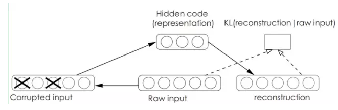
Denoising AutoEncodersé™å™ªè‡ªåŠ¨ç¼–ç 器:
é™å™ªè‡ªåŠ¨ç¼–ç 器DA是在自动编ç 器的基础上,è®ç»ƒæ•°æ®åŠ 入噪声,所以自动编ç 器必须å¦ä¹ 去去除这ç§å™ªå£°è€ŒèŽ·å¾—真æ£çš„æ²¡æœ‰è¢«å™ªå£°æ±¡æŸ“è¿‡çš„è¾“å…¥ã€‚å› æ¤ï¼Œè¿™å°±è¿«ä½¿ç¼–ç 器去å¦ä¹ 输入信å·çš„æ›´åŠ é²æ£’的表达,这也是它的泛化能力比一般编ç å™¨å¼ºçš„åŽŸå› ã€‚DAå¯ä»¥é€šè¿‡æ¢¯åº¦ä¸‹é™ç®—法去è®ç»ƒã€‚
9.2ã€Sparse Coding稀ç–ç¼–ç
如果我们把输出必须和输入相ç‰çš„é™åˆ¶æ”¾æ¾ï¼ŒåŒæ—¶åˆ©ç”¨çº¿æ€§ä»£æ•°ä¸åŸºçš„概念,å³O = a1Φ1 + a2Φ2+….+ anΦn, Φi是基,ai是系数,我们å¯ä»¥å¾—åˆ°è¿™æ ·ä¸€ä¸ªä¼˜åŒ–é—®é¢˜ï¼š
Min |I – O|,其ä¸I表示输入,O表示输出。
通过求解这个最优化å¼å,我们å¯ä»¥æ±‚得系数ai和基Φi,这些系数和基就是输入的å¦å¤–一ç§è¿‘似表达。
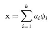
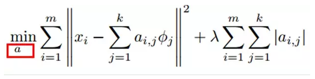
å› æ¤ï¼Œå®ƒä»¬å¯ä»¥ç”¨æ¥è¡¨è¾¾è¾“å…¥I,这个过程也是自动å¦ä¹ 得到的。如果我们在上述å¼åä¸ŠåŠ ä¸ŠL1çš„Regularityé™åˆ¶ï¼Œå¾—到:
Min |I – O| + u(|a1| + |a2| + … + |an |)
è¿™ç§æ–¹æ³•è¢«ç§°ä¸ºSparse Coding。通俗的说,就是将一个信å·è¡¨ç¤ºä¸ºä¸€ç»„基的线性组åˆï¼Œè€Œä¸”è¦æ±‚åªéœ€è¦è¾ƒå°‘çš„å‡ ä¸ªåŸºå°±å¯ä»¥å°†ä¿¡å·è¡¨ç¤ºå‡ºæ¥ã€‚“稀ç–性â€å®šä¹‰ä¸ºï¼šåªæœ‰å¾ˆå°‘çš„å‡ ä¸ªéžé›¶å…ƒç´ 或åªæœ‰å¾ˆå°‘çš„å‡ ä¸ªè¿œå¤§äºŽé›¶çš„å…ƒç´ ã€‚è¦æ±‚系数ai 是稀ç–çš„æ„æ€å°±æ˜¯è¯´ï¼šå¯¹äºŽä¸€ç»„输入å‘é‡ï¼Œæˆ‘们åªæƒ³æœ‰å°½å¯èƒ½å°‘çš„å‡ ä¸ªç³»æ•°è¿œå¤§äºŽé›¶ã€‚é€‰æ‹©ä½¿ç”¨å…·æœ‰ç¨€ç–性的分é‡æ¥è¡¨ç¤ºæˆ‘们的输入数æ®æ˜¯æœ‰åŽŸå› çš„ï¼Œå› ä¸ºç»å¤§å¤šæ•°çš„感官数æ®ï¼Œæ¯”如自然图åƒï¼Œå¯ä»¥è¢«è¡¨ç¤ºæˆå°‘é‡åŸºæœ¬å…ƒç´ çš„å åŠ ï¼Œåœ¨å›¾åƒä¸è¿™äº›åŸºæœ¬å…ƒç´ å¯ä»¥æ˜¯é¢æˆ–者线。åŒæ—¶ï¼Œæ¯”如与åˆçº§è§†è§‰çš®å±‚çš„ç±»æ¯”è¿‡ç¨‹ä¹Ÿå› æ¤å¾—到了æå‡ï¼ˆäººè„‘有大é‡çš„神ç»å…ƒï¼Œä½†å¯¹äºŽæŸäº›å›¾åƒæˆ–者边缘åªæœ‰å¾ˆå°‘的神ç»å…ƒå…´å¥‹ï¼Œå…¶ä»–都处于抑制状æ€ï¼‰ã€‚
稀ç–ç¼–ç 算法是一ç§æ— 监ç£å¦ä¹ 方法,它用æ¥å¯»æ‰¾ä¸€ç»„“超完备â€åŸºå‘é‡æ¥æ›´é«˜æ•ˆåœ°è¡¨ç¤ºæ ·æœ¬æ•°æ®ã€‚虽然形如主æˆåˆ†åˆ†æžæŠ€æœ¯ï¼ˆPCA)能使我们方便地找到一组“完备â€åŸºå‘é‡ï¼Œä½†æ˜¯è¿™é‡Œæˆ‘们想è¦åšçš„是找到一组“超完备â€åŸºå‘é‡æ¥è¡¨ç¤ºè¾“å…¥å‘é‡ï¼ˆä¹Ÿå°±æ˜¯è¯´ï¼ŒåŸºå‘é‡çš„个数比输入å‘é‡çš„ç»´æ•°è¦å¤§ï¼‰ã€‚超完备基的好处是它们能更有效地找出éšå«åœ¨è¾“入数æ®å†…部的结构与模å¼ã€‚然而,对于超完备基æ¥è¯´ï¼Œç³»æ•°aiä¸å†ç”±è¾“å…¥å‘é‡å”¯ä¸€ç¡®å®šã€‚å› æ¤ï¼Œåœ¨ç¨€ç–ç¼–ç 算法ä¸ï¼Œæˆ‘们å¦åŠ äº†ä¸€ä¸ªè¯„åˆ¤æ ‡å‡†â€œç¨€ç–性â€æ¥è§£å†³å› 超完备而导致的退化(degeneracy)问题。

比如在图åƒçš„Feature Extraction的最底层è¦åšEdge Detector的生æˆï¼Œé‚£ä¹ˆè¿™é‡Œçš„工作就是从Natural Imagesä¸randomly选å–一些å°patch,通过这些patch生æˆèƒ½å¤Ÿæ述他们的“基â€ï¼Œä¹Ÿå°±æ˜¯å³è¾¹çš„88=64个basis组æˆçš„basis,然åŽç»™å®šä¸€ä¸ªtest patch, 我们å¯ä»¥æŒ‰ç…§ä¸Šé¢çš„å¼å通过basis的线性组åˆå¾—到,而sparse matrix就是a,下图ä¸çš„aä¸æœ‰64个维度,其ä¸éžé›¶é¡¹åªæœ‰3个,故称“sparseâ€ã€‚
这里å¯èƒ½å¤§å®¶ä¼šæœ‰ç–‘问,为什么把底层作为Edge Detector呢?上层åˆæ˜¯ä»€ä¹ˆå‘¢ï¼Ÿè¿™é‡Œåšä¸ªç®€å•è§£é‡Šå¤§å®¶å°±ä¼šæ˜Žç™½ï¼Œä¹‹æ‰€ä»¥æ˜¯Edge Detectoræ˜¯å› ä¸ºä¸åŒæ–¹å‘çš„Edge就能够æ述出整幅图åƒï¼Œæ‰€ä»¥ä¸åŒæ–¹å‘çš„Edge自然就是图åƒçš„basis了……而上一层的basis组åˆçš„结果,上上层åˆæ˜¯ä¸Šä¸€å±‚的组åˆbasis……(就是上é¢ç¬¬å››éƒ¨åˆ†çš„æ—¶å€™å’±ä»¬è¯´çš„é‚£æ ·ï¼‰
Sparse coding分为两个部分:
1)Trainingé˜¶æ®µï¼šç»™å®šä¸€ç³»åˆ—çš„æ ·æœ¬å›¾ç‰‡[x1, x 2, …],我们需è¦å¦ä¹ 得到一组基[Φ1, Φ2, …],也就是å—典。
稀ç–ç¼–ç 是k-means算法的å˜ä½“,其è®ç»ƒè¿‡ç¨‹ä¹Ÿå·®ä¸å¤šï¼ˆEM算法的æ€æƒ³ï¼šå¦‚æžœè¦ä¼˜åŒ–çš„ç›®æ ‡å‡½æ•°åŒ…å«ä¸¤ä¸ªå˜é‡ï¼Œå¦‚L(W, B),那么我们å¯ä»¥å…ˆå›ºå®šW,调整B使得L最å°ï¼Œç„¶åŽå†å›ºå®šB,调整W使L最å°ï¼Œè¿™æ ·è¿ä»£äº¤æ›¿ï¼Œä¸æ–å°†L推å‘最å°å€¼ã€‚
è®ç»ƒè¿‡ç¨‹å°±æ˜¯ä¸€ä¸ªé‡å¤è¿ä»£çš„过程,按上é¢æ‰€è¯´ï¼Œæˆ‘们交替的更改a和Φ使得下é¢è¿™ä¸ªç›®æ ‡å‡½æ•°æœ€å°ã€‚

æ¯æ¬¡è¿ä»£åˆ†ä¸¤æ¥ï¼š
a)固定å—典Φ[k],然åŽè°ƒæ•´a[k],使得上å¼ï¼Œå³ç›®æ ‡å‡½æ•°æœ€å°ï¼ˆå³è§£LASSO问题)。
b)然åŽå›ºå®šä½a [k],调整Φ [k],使得上å¼ï¼Œå³ç›®æ ‡å‡½æ•°æœ€å°ï¼ˆå³è§£å‡¸QP问题)。
ä¸æ–è¿ä»£ï¼Œç›´è‡³æ”¶æ•›ã€‚è¿™æ ·å°±å¯ä»¥å¾—到一组å¯ä»¥è‰¯å¥½è¡¨ç¤ºè¿™ä¸€ç³»åˆ—x的基,也就是å—典。
2)Coding阶段:给定一个新的图片x,由上é¢å¾—到的å—典,通过解一个LASSO问题得到稀ç–å‘é‡a。这个稀ç–å‘é‡å°±æ˜¯è¿™ä¸ªè¾“å…¥å‘é‡x的一个稀ç–表达了。
E.g:
9.3ã€Restricted Boltzmann Machine (RBM)é™åˆ¶æ³¢å°”兹曼机
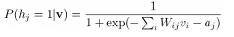
å‡è®¾æœ‰ä¸€ä¸ªäºŒéƒ¨å›¾ï¼Œæ¯ä¸€å±‚的节点之间没有链接,一层是å¯è§†å±‚,å³è¾“入数æ®å±‚(v),一层是éšè—层(h),如果å‡è®¾æ‰€æœ‰çš„节点都是éšæœºäºŒå€¼å˜é‡èŠ‚点(åªèƒ½å–0或者1值),åŒæ—¶å‡è®¾å…¨æ¦‚率分布p(v,h)满足Boltzmann 分布,我们称这个模型是Restricted BoltzmannMachine (RBM)。

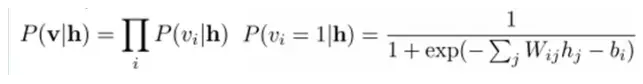
下é¢æˆ‘们æ¥çœ‹çœ‹ä¸ºä»€ä¹ˆå®ƒæ˜¯Deep Learningæ–¹æ³•ã€‚é¦–å…ˆï¼Œè¿™ä¸ªæ¨¡åž‹å› ä¸ºæ˜¯äºŒéƒ¨å›¾ï¼Œæ‰€ä»¥åœ¨å·²çŸ¥v的情况下,所有的éšè—节点之间是æ¡ä»¶ç‹¬ç«‹çš„ï¼ˆå› ä¸ºèŠ‚ç‚¹ä¹‹é—´ä¸å˜åœ¨è¿žæŽ¥ï¼‰ï¼Œå³p(h|v)=p(h1|v)…p(hn|v)。åŒç†ï¼Œåœ¨å·²çŸ¥éšè—层h的情况下,所有的å¯è§†èŠ‚点都是æ¡ä»¶ç‹¬ç«‹çš„。åŒæ—¶åˆç”±äºŽæ‰€æœ‰çš„vå’Œh满足Boltzmann åˆ†å¸ƒï¼Œå› æ¤ï¼Œå½“输入v的时候,通过p(h|v) å¯ä»¥å¾—到éšè—层h,而得到éšè—层h之åŽï¼Œé€šè¿‡p(v|h)åˆèƒ½å¾—到å¯è§†å±‚,通过调整å‚数,我们就是è¦ä½¿å¾—从éšè—层得到的å¯è§†å±‚v1与原æ¥çš„å¯è§†å±‚vå¦‚æžœä¸€æ ·ï¼Œé‚£ä¹ˆå¾—åˆ°çš„éšè—层就是å¯è§†å±‚å¦å¤–一ç§è¡¨è¾¾ï¼Œå› æ¤éšè—层å¯ä»¥ä½œä¸ºå¯è§†å±‚输入数æ®çš„特å¾ï¼Œæ‰€ä»¥å®ƒå°±æ˜¯ä¸€ç§Deep Learning方法。

如何è®ç»ƒå‘¢ï¼Ÿä¹Ÿå°±æ˜¯å¯è§†å±‚节点和éšèŠ‚点间的æƒå€¼æ€Žä¹ˆç¡®å®šå‘¢ï¼Ÿæˆ‘们需è¦åšä¸€äº›æ•°å¦åˆ†æžã€‚也就是模型了。
è”åˆç»„æ€ï¼ˆjointconfiguration)的能é‡å¯ä»¥è¡¨ç¤ºä¸ºï¼š
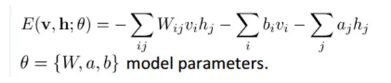
而æŸä¸ªç»„æ€çš„è”åˆæ¦‚率分布å¯ä»¥é€šè¿‡Boltzmann 分布(和这个组æ€çš„能é‡ï¼‰æ¥ç¡®å®šï¼š
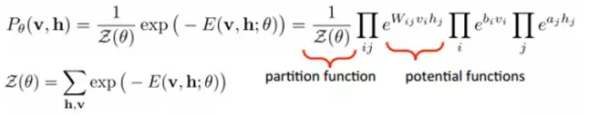
å› ä¸ºéšè—节点之间是æ¡ä»¶ç‹¬ç«‹çš„ï¼ˆå› ä¸ºèŠ‚ç‚¹ä¹‹é—´ä¸å˜åœ¨è¿žæŽ¥ï¼‰ï¼Œå³ï¼š
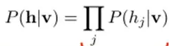
然åŽæˆ‘们å¯ä»¥æ¯”较容易(对上å¼è¿›è¡Œå› å分解Factorizes)得到在给定å¯è§†å±‚v的基础上,éšå±‚第j个节点为1或者为0的概率:
åŒç†ï¼Œåœ¨ç»™å®šéšå±‚h的基础上,å¯è§†å±‚第i个节点为1或者为0的概率也å¯ä»¥å®¹æ˜“得到:
给定一个满足独立åŒåˆ†å¸ƒçš„æ ·æœ¬é›†ï¼šD={v(1), v(2),…, v(N)},我们需è¦å¦ä¹ å‚数θ={W,a,b}。
我们最大化以下对数似然函数(最大似然估计:对于æŸä¸ªæ¦‚率模型,我们需è¦é€‰æ‹©ä¸€ä¸ªå‚数,让我们当å‰çš„è§‚æµ‹æ ·æœ¬çš„æ¦‚çŽ‡æœ€å¤§ï¼‰ï¼š
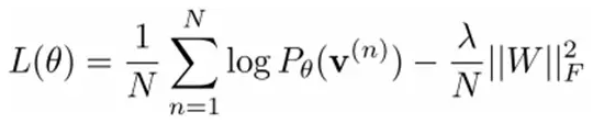
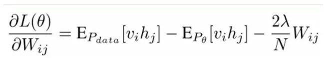
也就是对最大对数似然函数求导,就å¯ä»¥å¾—到L最大时对应的å‚æ•°W了。
如果,我们把éšè—å±‚çš„å±‚æ•°å¢žåŠ ï¼Œæˆ‘ä»¬å¯ä»¥å¾—到Deep Boltzmann Machine(DBM);如果我们在é è¿‘å¯è§†å±‚的部分使用è´å¶æ–¯ä¿¡å¿µç½‘络(å³æœ‰å‘图模型,当然这里ä¾ç„¶é™åˆ¶å±‚ä¸èŠ‚点之间没有链接),而在最远离å¯è§†å±‚的部分使用Restricted Boltzmann Machine,我们å¯ä»¥å¾—到DeepBelief Net(DBN)。

9.4ã€Deep Belief Networks深信度网络
DBNs是一个概率生æˆæ¨¡åž‹ï¼Œä¸Žä¼ 统的判别模型的神ç»ç½‘络相对,生æˆæ¨¡åž‹æ˜¯å»ºç«‹ä¸€ä¸ªè§‚察数æ®å’Œæ ‡ç¾ä¹‹é—´çš„è”åˆåˆ†å¸ƒï¼Œå¯¹P(Observation|Label)å’ŒP(Label|Observation)都åšäº†è¯„估,而判别模型仅仅而已评估了åŽè€…,也就是P(Label|Observation)。对于在深度神ç»ç½‘ç»œåº”ç”¨ä¼ ç»Ÿçš„BP算法的时候,DBNsé‡åˆ°äº†ä»¥ä¸‹é—®é¢˜ï¼š
(1)需è¦ä¸ºè®ç»ƒæä¾›ä¸€ä¸ªæœ‰æ ‡ç¾çš„æ ·æœ¬é›†ï¼›
(2)å¦ä¹ 过程较慢;
(3)ä¸é€‚当的å‚数选择会导致å¦ä¹ 收敛于局部最优解。
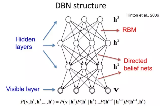
DBNs由多个é™åˆ¶çŽ»å°”兹曼机(Restricted Boltzmann Machines)层组æˆï¼Œä¸€ä¸ªå…¸åž‹çš„神ç»ç½‘络类型如图三所示。这些网络被“é™åˆ¶â€ä¸ºä¸€ä¸ªå¯è§†å±‚和一个éšå±‚,层间å˜åœ¨è¿žæŽ¥ï¼Œä½†å±‚内的å•å…ƒé—´ä¸å˜åœ¨è¿žæŽ¥ã€‚éšå±‚å•å…ƒè¢«è®ç»ƒåŽ»æ•æ‰åœ¨å¯è§†å±‚表现出æ¥çš„高阶数æ®çš„相关性。
首先,先ä¸è€ƒè™‘最顶构æˆä¸€ä¸ªè”想记忆(associative memory)的两层,一个DBN的连接是通过自顶å‘下的生æˆæƒå€¼æ¥æŒ‡å¯¼ç¡®å®šçš„,RBMså°±åƒä¸€ä¸ªå»ºç‘å—ä¸€æ ·ï¼Œç›¸æ¯”ä¼ ç»Ÿå’Œæ·±åº¦åˆ†å±‚çš„sigmoid信念网络,它能易于连接æƒå€¼çš„å¦ä¹ 。
最开始的时候,通过一个éžç›‘ç£è´ªå©ªé€å±‚方法去预è®ç»ƒèŽ·å¾—生æˆæ¨¡åž‹çš„æƒå€¼ï¼Œéžç›‘ç£è´ªå©ªé€å±‚方法被Hintonè¯æ˜Žæ˜¯æœ‰æ•ˆçš„,并被其称为对比分æ§ï¼ˆcontrastive divergence)。
在这个è®ç»ƒé˜¶æ®µï¼Œåœ¨å¯è§†å±‚会产生一个å‘é‡vï¼Œé€šè¿‡å®ƒå°†å€¼ä¼ é€’åˆ°éšå±‚。å过æ¥ï¼Œå¯è§†å±‚的输入会被éšæœºçš„选择,以å°è¯•åŽ»é‡æž„原始的输入信å·ã€‚最åŽï¼Œè¿™äº›æ–°çš„å¯è§†çš„神ç»å…ƒæ¿€æ´»å•å…ƒå°†å‰å‘ä¼ é€’é‡æž„éšå±‚激活å•å…ƒï¼ŒèŽ·å¾—h(在è®ç»ƒè¿‡ç¨‹ä¸ï¼Œé¦–先将å¯è§†å‘é‡å€¼æ˜ å°„ç»™éšå•å…ƒï¼›ç„¶åŽå¯è§†å•å…ƒç”±éšå±‚å•å…ƒé‡å»ºï¼›è¿™äº›æ–°å¯è§†å•å…ƒå†æ¬¡æ˜ å°„ç»™éšå•å…ƒï¼Œè¿™æ ·å°±èŽ·å–æ–°çš„éšå•å…ƒã€‚执行这ç§åå¤æ¥éª¤å«åšå‰å¸ƒæ–¯é‡‡æ ·ï¼‰ã€‚这些åŽé€€å’Œå‰è¿›çš„æ¥éª¤å°±æ˜¯æˆ‘们熟悉的Gibbsé‡‡æ ·ï¼Œè€Œéšå±‚激活å•å…ƒå’Œå¯è§†å±‚输入之间的相关性差别就作为æƒå€¼æ›´æ–°çš„主è¦ä¾æ®ã€‚
è®ç»ƒæ—¶é—´ä¼šæ˜¾è‘—çš„å‡å°‘ï¼Œå› ä¸ºåªéœ€è¦å•ä¸ªæ¥éª¤å°±å¯ä»¥æŽ¥è¿‘最大似然å¦ä¹ ã€‚å¢žåŠ è¿›ç½‘ç»œçš„æ¯ä¸€å±‚都会改进è®ç»ƒæ•°æ®çš„对数概率,我们å¯ä»¥ç†è§£ä¸ºè¶Šæ¥è¶ŠæŽ¥è¿‘能é‡çš„真实表达。这个有æ„ä¹‰çš„æ‹“å±•ï¼Œå’Œæ— æ ‡ç¾æ•°æ®çš„使用,是任何一个深度å¦ä¹ åº”ç”¨çš„å†³å®šæ€§çš„å› ç´ ã€‚

在最高两层,æƒå€¼è¢«è¿žæŽ¥åˆ°ä¸€èµ·ï¼Œè¿™æ ·æ›´ä½Žå±‚的输出将会æ供一个å‚考的线索或者关è”ç»™é¡¶å±‚ï¼Œè¿™æ ·é¡¶å±‚å°±ä¼šå°†å…¶è”系到它的记忆内容。而我们最关心的,最åŽæƒ³å¾—到的就是判别性能,例如分类任务里é¢ã€‚
在预è®ç»ƒåŽï¼ŒDBNå¯ä»¥é€šè¿‡åˆ©ç”¨å¸¦æ ‡ç¾æ•°æ®ç”¨BP算法去对判别性能åšè°ƒæ•´ã€‚åœ¨è¿™é‡Œï¼Œä¸€ä¸ªæ ‡ç¾é›†å°†è¢«é™„åŠ åˆ°é¡¶å±‚ï¼ˆæŽ¨å¹¿è”想记忆),通过一个自下å‘上的,å¦ä¹ 到的识别æƒå€¼èŽ·å¾—一个网络的分类é¢ã€‚这个性能会比å•çº¯çš„BP算法è®ç»ƒçš„网络好。这å¯ä»¥å¾ˆç›´è§‚的解释,DBNsçš„BP算法åªéœ€è¦å¯¹æƒå€¼å‚数空间进行一个局部的æœç´¢ï¼Œè¿™ç›¸æ¯”å‰å‘神ç»ç½‘络æ¥è¯´ï¼Œè®ç»ƒæ˜¯è¦å¿«çš„,而且收敛的时间也少。
DBNsçš„çµæ´»æ€§ä½¿å¾—它的拓展比较容易。一个拓展就是å·ç§¯DBNs(Convolutional Deep Belief Networks(CDBNs))。DBNs并没有考虑到图åƒçš„2维结构信æ¯ï¼Œå› 为输入是简å•çš„从一个图åƒçŸ©é˜µä¸€ç»´å‘é‡åŒ–的。而CDBNs就是考虑到了这个问题,它利用邻域åƒç´ 的空域关系,通过一个称为å·ç§¯RBMs的模型区达到生æˆæ¨¡åž‹çš„å˜æ¢ä¸å˜æ€§ï¼Œè€Œä¸”å¯ä»¥å®¹æ˜“å¾—å˜æ¢åˆ°é«˜ç»´å›¾åƒã€‚DBNs并没有明确地处ç†å¯¹è§‚察å˜é‡çš„时间è”系的å¦ä¹ 上,虽然目å‰å·²ç»æœ‰è¿™æ–¹é¢çš„ç ”ç©¶ï¼Œä¾‹å¦‚å †å 时间RBMs,以æ¤ä¸ºæŽ¨å¹¿ï¼Œæœ‰åºåˆ—å¦ä¹ çš„dubbed temporal convolutionmachines,这ç§åºåˆ—å¦ä¹ 的应用,给è¯éŸ³ä¿¡å·å¤„ç†é—®é¢˜å¸¦æ¥äº†ä¸€ä¸ªè®©äººæ¿€åŠ¨çš„未æ¥ç ”究方å‘。
ç›®å‰ï¼Œå’ŒDBNsæœ‰å…³çš„ç ”ç©¶åŒ…æ‹¬å †å 自动编ç å™¨ï¼Œå®ƒæ˜¯é€šè¿‡ç”¨å †å 自动编ç 器æ¥æ›¿æ¢ä¼ 统DBNs里é¢çš„RBMs。这就使得å¯ä»¥é€šè¿‡åŒæ ·çš„规则æ¥è®ç»ƒäº§ç”Ÿæ·±åº¦å¤šå±‚神ç»ç½‘络架构,但它缺少层的å‚æ•°åŒ–çš„ä¸¥æ ¼è¦æ±‚。与DBNsä¸åŒï¼Œè‡ªåŠ¨ç¼–ç å™¨ä½¿ç”¨åˆ¤åˆ«æ¨¡åž‹ï¼Œè¿™æ ·è¿™ä¸ªç»“æž„å°±å¾ˆéš¾é‡‡æ ·è¾“å…¥é‡‡æ ·ç©ºé—´ï¼Œè¿™å°±ä½¿å¾—ç½‘ç»œæ›´éš¾æ•æ‰å®ƒçš„内部表达。但是,é™å™ªè‡ªåŠ¨ç¼–ç 器å´èƒ½å¾ˆå¥½çš„é¿å…è¿™ä¸ªé—®é¢˜ï¼Œå¹¶ä¸”æ¯”ä¼ ç»Ÿçš„DBNs更优。它通过在è®ç»ƒè¿‡ç¨‹æ·»åŠ éšæœºçš„æ±¡æŸ“å¹¶å †å 产生场泛化性能。è®ç»ƒå•ä¸€çš„é™å™ªè‡ªåŠ¨ç¼–ç 器的过程和RBMsè®ç»ƒç”Ÿæˆæ¨¡åž‹çš„è¿‡ç¨‹ä¸€æ ·ã€‚
| åã€æ€»ç»“与展望
1)Deep learning总结
深度å¦ä¹ 是关于自动å¦ä¹ è¦å»ºæ¨¡çš„æ•°æ®çš„潜在(éšå«ï¼‰åˆ†å¸ƒçš„多层(å¤æ‚)表达的算法。æ¢å¥è¯æ¥è¯´ï¼Œæ·±åº¦å¦ä¹ 算法自动的æå–分类需è¦çš„低层次或者高层次特å¾ã€‚高层次特å¾ï¼Œä¸€æ˜¯æŒ‡è¯¥ç‰¹å¾å¯ä»¥åˆ†çº§ï¼ˆå±‚次)地ä¾èµ–其他特å¾ï¼Œä¾‹å¦‚:对于机器视觉,深度å¦ä¹ 算法从原始图åƒåŽ»å¦ä¹ 得到它的一个低层次表达,例如边缘检测器,å°æ³¢æ»¤æ³¢å™¨ç‰ï¼Œç„¶åŽåœ¨è¿™äº›ä½Žå±‚次表达的基础上å†å»ºç«‹è¡¨è¾¾ï¼Œä¾‹å¦‚这些低层次表达的线性或者éžçº¿æ€§ç»„åˆï¼Œç„¶åŽé‡å¤è¿™ä¸ªè¿‡ç¨‹ï¼Œæœ€åŽå¾—到一个高层次的表达。
Deep learning能够得到更好地表示数æ®çš„feature,åŒæ—¶ç”±äºŽæ¨¡åž‹çš„层次ã€å‚数很多,capacityè¶³å¤Ÿï¼Œå› æ¤ï¼Œæ¨¡åž‹æœ‰èƒ½åŠ›è¡¨ç¤ºå¤§è§„模数æ®ï¼Œæ‰€ä»¥å¯¹äºŽå›¾åƒã€è¯éŸ³è¿™ç§ç‰¹å¾ä¸æ˜Žæ˜¾ï¼ˆéœ€è¦æ‰‹å·¥è®¾è®¡ä¸”很多没有直观物ç†å«ä¹‰ï¼‰çš„问题,能够在大规模è®ç»ƒæ•°æ®ä¸Šå–得更好的效果。æ¤å¤–,从模å¼è¯†åˆ«ç‰¹å¾å’Œåˆ†ç±»å™¨çš„角度,deep learning框架将feature和分类器结åˆåˆ°ä¸€ä¸ªæ¡†æž¶ä¸ï¼Œç”¨æ•°æ®åŽ»å¦ä¹ feature,在使用ä¸å‡å°‘了手工设计feature的巨大工作é‡ï¼ˆè¿™æ˜¯ç›®å‰å·¥ä¸šç•Œå·¥ç¨‹å¸ˆä»˜å‡ºåŠªåŠ›æœ€å¤šçš„æ–¹é¢ï¼‰ï¼Œå› æ¤ï¼Œä¸ä»…仅效果å¯ä»¥æ›´å¥½ï¼Œè€Œä¸”,使用起æ¥ä¹Ÿæœ‰å¾ˆå¤šæ–¹ä¾¿ä¹‹å¤„ï¼Œå› æ¤ï¼Œæ˜¯å分值得关注的一套框架,æ¯ä¸ªåšML的人都应该关注了解一下。
当然,deep learning本身也ä¸æ˜¯å®Œç¾Žçš„,也ä¸æ˜¯è§£å†³ä¸–间任何ML问题的利器,ä¸åº”è¯¥è¢«æ”¾å¤§åˆ°ä¸€ä¸ªæ— æ‰€ä¸èƒ½çš„程度。
2)Deep learning未æ¥
深度å¦ä¹ ç›®å‰ä»æœ‰å¤§é‡å·¥ä½œéœ€è¦ç ”究。目å‰çš„关注点还是从机器å¦ä¹ 的领域借鉴一些å¯ä»¥åœ¨æ·±åº¦å¦ä¹ 使用的方法特别是é™ç»´é¢†åŸŸã€‚例如:目å‰ä¸€ä¸ªå·¥ä½œå°±æ˜¯ç¨€ç–ç¼–ç ,通过压缩感知ç†è®ºå¯¹é«˜ç»´æ•°æ®è¿›è¡Œé™ç»´ï¼Œä½¿å¾—éžå¸¸å°‘çš„å…ƒç´ çš„å‘é‡å°±å¯ä»¥ç²¾ç¡®çš„代表原æ¥çš„高维信å·ã€‚å¦ä¸€ä¸ªä¾‹å就是åŠç›‘ç£æµè¡Œå¦ä¹ ,通过测é‡è®ç»ƒæ ·æœ¬çš„相似性,将高维数æ®çš„è¿™ç§ç›¸ä¼¼æ€§æŠ•å½±åˆ°ä½Žç»´ç©ºé—´ã€‚å¦å¤–一个比较鼓舞人心的方å‘就是evolutionary programming approaches(é—ä¼ ç¼–ç¨‹æ–¹æ³•ï¼‰ï¼Œå®ƒå¯ä»¥é€šè¿‡æœ€å°åŒ–工程能é‡åŽ»è¿›è¡Œæ¦‚念性自适应å¦ä¹ 和改å˜æ ¸å¿ƒæž¶æž„。
Deep learningè¿˜æœ‰å¾ˆå¤šæ ¸å¿ƒçš„é—®é¢˜éœ€è¦è§£å†³ï¼š
(1)对于一个特定的框架,对于多少维的输入它å¯ä»¥è¡¨çŽ°å¾—较优(如果是图åƒï¼Œå¯èƒ½æ˜¯ä¸Šç™¾ä¸‡ç»´ï¼‰ï¼Ÿ
(2)对æ•æ‰çŸæ—¶æˆ–者长时间的时间ä¾èµ–,哪ç§æž¶æž„æ‰æ˜¯æœ‰æ•ˆçš„?
(3)如何对于一个给定的深度å¦ä¹ 架构,èžåˆå¤šç§æ„ŸçŸ¥çš„ä¿¡æ¯ï¼Ÿ
(4)有什么æ£ç¡®çš„机ç†å¯ä»¥åŽ»å¢žå¼ºä¸€ä¸ªç»™å®šçš„深度å¦ä¹ 架构,以改进其é²æ£’性和对æ‰æ›²å’Œæ•°æ®ä¸¢å¤±çš„ä¸å˜æ€§ï¼Ÿ
(5)模型方é¢æ˜¯å¦æœ‰å…¶ä»–更为有效且有ç†è®ºä¾æ®çš„深度模型å¦ä¹ 算法?
探索新的特å¾æå–æ¨¡åž‹æ˜¯å€¼å¾—æ·±å…¥ç ”ç©¶çš„å†…å®¹ã€‚æ¤å¤–有效的å¯å¹¶è¡Œè®ç»ƒç®—æ³•ä¹Ÿæ˜¯å€¼å¾—ç ”ç©¶çš„ä¸€ä¸ªæ–¹å‘。当å‰åŸºäºŽæœ€å°æ‰¹å¤„ç†çš„éšæœºæ¢¯åº¦ä¼˜åŒ–算法很难在多计算机ä¸è¿›è¡Œå¹¶è¡Œè®ç»ƒã€‚通常办法是利用图形处ç†å•å…ƒåŠ 速å¦ä¹ 过程。然而å•ä¸ªæœºå™¨GPU对大规模数æ®è¯†åˆ«æˆ–相似任务数æ®é›†å¹¶ä¸é€‚用。在深度å¦ä¹ 应用拓展方é¢ï¼Œå¦‚何åˆç†å……分利用深度å¦ä¹ åœ¨å¢žå¼ºä¼ ç»Ÿå¦ä¹ 算法的性能ä»æ˜¯ç›®å‰å„é¢†åŸŸçš„ç ”ç©¶é‡ç‚¹ã€‚
本文转自阅é¢ç§‘技专注深度å¦ä¹ 和嵌入å¼è§†è§‰çš„人工智能平å°ï¼Œå¦‚需转载请è”系原作者。
Strain/flex Reliefs And Grommets
the power Connectors we provide overmolding solutions and modular tooling.
We also offer to the OEM and distributor users a diversified line of strain / flex reliefs and grommets, such as Solid, Solid-Rib, Uniflex, Multiflex, in standard off the shelf or custom designs.
Overmolding the power connectors offers significant opportunities for cable improvements with higher pull strength not available with conventional backshells. Our technical staff is ready to help you from design and prototyping to small production run, assistance, and training.
Our team is ready to help with any of the following power connectors projects: overmolding mini fit jr. and mini-fit sr. connectors, , overmolded cables with micro fit terminations, sabre molded cable asemblies, amp duac overmolded power connectors, mate-n-lock power cables, power connector overmolding services, power connector molding, design and prototype of power cables across the board, small run molded power connecotrs , molded cable manufacturing, overmolding connectors for any power applications
Strain Reliefs And Grommets,Flex Reliefs And Grommets,Cable Strain Reliefs,Cable Flex Reliefs,Cable Grommets,Molded Strain Relief
ETOP WIREHARNESS LIMITED , https://www.etopwireharness.com